5. EXAMPLE REACTION SYSTEMS¶

This section demonstrates how several different multi-species reaction systems of interest can be modeled with EPANET-MSX.

5.1. Multi-Source Chlorine Decay¶

Multi-source networks present problems modeling a single species, such as free chlorine, when the decay rates observed in the source waters vary quite significantly. As the sources blend differently throughout the network, it becomes difficult to assign a single decay coefficient that accurately reflects the decay rate observed in the blended water. Consider the distribution system shown in Fig. 5.1 that is served by two different sources. The network has been color-coded to show the average fraction of water in each pipe that originates from the River (Source 1).

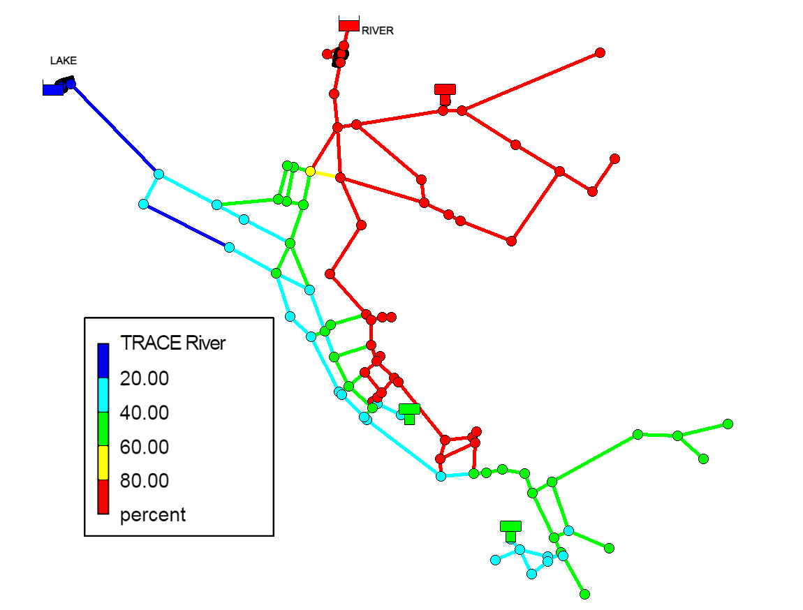
Fig. 5.1 Example of a two-source water distribution system showing the average percent of water originating from the River source¶

Assume that free chlorine reacts in the bulk flow along a pipe according to the following first-order rate expression:

(5.1)¶\[\begin{aligned} {d {C} \over d {t}} = {-kC} \end{aligned}\]

where \(C\) is the concentration of free chlorine at time \(t\) and \(k\) is a reaction rate constant. Now suppose that when analyzed separately in bottle tests, water from Source 1 has a \(k\) = 1.3 days^-1 while Source 2’s water has \(k\) = 17.7 days^-1. The issue becomes one of determining a \({k}\)-value for each pipe of the network that will reflect the proper reactivity of the blended water from both sources.

One approach to reconciling the vastly different chlorine decay constants in this example, without introducing a more complex chlorine decay mechanism that attempts to represent the different reactivity of the total organics from the two sources, is to assume that at any time the chlorine decay constant within a pipe is given by a weighted average of the two source values, where the weights are the fraction of each source water present in the pipe. These fractions can be deduced by introducing a fictitious conservative tracer compound at Source 1, denoted as T1, whose concentration is fixed at a constant 1.0 \(mg/L\). Then at any point in the network the fraction of water from Source 1 would be the concentration of T1 while the fraction from Source 2 would be 1.0 minus that value. The resulting chlorine decay model now consists of two-species – a tracer species \(T1\) and a free chlorine species \(C\). The first-order decay constant k for any pipe in the system would be given by:

(5.2)¶\[\begin{aligned} k = 1.3{T1}+17.7{(1.0-T1)} \end{aligned}\]

while the system reaction dynamics would be expressed by:

(5.3)¶\[\begin{aligned} {d {T1} \over d {t}} = 0 \end{aligned}\]

(5.4)¶\[\begin{aligned} {d {C} \over d {t}} = {{-(1.3{T1}+17.7{(1.0-T1)})}C} \end{aligned}\]

Listing 5.1 is the MSX input file that defines this model for a network where the two source nodes are represented as reservoirs with ID names “1” and “2”, respectively. Note that it contains no surface species, no equilibrium species, and assumes that a constant chlorine concentration of 1.2 \(mg/L\) is maintained at each source.

Listing 5.1 EPANET-MSX input file for modeling two-source chlorine decay¶

[OPTIONS]
  AREA_UNITS  FT2
  RATE_UNITS  DAY
  SOLVER      RK5
  TIMESTEP    300

[SPECIES]
  BULK  T1    MG         ;Source 1 tracer
  BULK  CL2   MG         ;Free chlorine

[COEFFICIENTS]
  CONSTANT  k1  1.3      ;Source 1 decay coeff.
  CONSTANT  k2  17.7     ;Source 2 decay coeff.

[PIPES]
  ;T1 is conservative
  RATE  T1   0

  ;CL2 has first order decay
  RATE  CL2  –(k1*T1 + k2*(1-T1))*CL2

[QUALITY]
  ;Initial conditions (= 0 if not specified here)
  NODE   1      T1   1.0 
  NODE   1      CL2  1.2
  NODE   2      CL2  1.2   

5.2. Decay and Dispersion Modeling of Chlorine¶

This example illustrates how to use EPANET MSX to model the advection, self-decay, and dispersion of the chlorine within a water distrinution system. The chlorine decay model is the same as the first order decay model in EPANET 2.2. Both bulk decay and wall decay are considered in this example.

The rate of chlorine first-order decay in bulk water is described as:

\[r_b = -K_b*C\]

where \(K_b\) = a bulk reaction constant and \(r_b\) = the bulk decay rate.

For first-order decay, the rate of a pipe wall reaction is expressed as:

\[r_w = -\frac{ 2 K_w K_f C } { R (K_w + K_f) }\]

where \(K_w\) = wall reaction rate constant (length/time), \(r_w\) = wall reaction rate, \(K_f\) = mass transfer coefficient (length/time), and \(R\) = pipe radius.

Mass transfer coefficients are expressed in terms of a dimensionless Sherwood number (\(Sh\)):

\[{K}_{f} = Sh \frac{\mathcal{D}}{2R}\]

in which \(\mathcal{D}\) = the molecular diffusivity of the species being transported (length ² /time) and \(R\) = pipe radius. In fully developed laminar flow, the average Sherwood number along the length of a pipe can be expressed as

\[Sh = 3.65 + \frac{0.0668 ( 2R/L )Re\ Sc} {1 + 0.04{ [ ( 2R/L )Re\ Sc ]}^{2/3}}\]

in which \(Re\) = Reynolds number and \(Sc\) = Schmidt number (kinematic viscosity of water divided by the diffusivity of the chemical).

For turbulent flow, the empirical correlation is used:

\[Sh = 0.0149{Re}^{0.88}{Sc}^{1/3}\]

Listing 5.2 is the MSX input file that defines this model for the EPANET example model NET2. In this model, \(K_b = 0.3 /day\) and \(K_w = 1.0 ft/day\). The Schmidt number is specified in the file as a dimensionless constant of 846.15, based on the kinematic viscosity of water and molecular diffusivity of chlorine. The terms SHt and SHl are defined as the Sherwood number under the turbulent and laminar flow condition, respectively. STEP is the step function defined inside the EPANET MSX: STEP (x<=0 ? 0 : 1). This function determines the Sherwood number based on the Reynolds number (\(Re\)). As described in Section 4.5, \(D\), \(Len\), and \(Re\) are reserved keywords for the Reynolds number, pipe diameter, and pipe length, respectively. The molecular diffusivity of chlorine is \(1.3 \times 10^{-8} ft^2/s\). Since the rate unit here is day, it is correspondingly converted to \(0.00112 ft^2/day\) for the caluclation of \(K_f\).

In order to model the longitudinal dispersion, the relative diffusivity of chlorine is defined in the [DIFFUSIVITY] section. It is simply 1.0 (\(1.3 \times 10^{-8} ft^2/s\)) here. It should be noted that the molecular diffusivity used in the calculation of \(K_f\) is to model the transport of chlorine from the bulk water to the pipe wall, while the diffusivity specified in the [DIFFUSIVITY] section is to model the longitudinal dispersion of chlorine. If the relative diffsusity of chlorine is not defined, longitudinal dispersion is ignored and the model will be the same as the EPANET’s first-order decay model.

Listing 5.2 EPANET-MSX input file for modeling chlorine decay and dispersion (example2.msx)¶

[TITLE]

NET2 Chlorine Decay and Dispersion

[OPTIONS]

AREA_UNITS  FT2
RATE_UNITS  DAY
SOLVER      EUL
TIMESTEP    60
RTOL        0.001
ATOL        0.001

[SPECIES]

BULK        CL2    MG  0.01 0.001


[COEFFICIENTS]

PARAMETER  Kb   0.3
PARAMETER  Kw   1.0
CONSTANT     Sc    846.15

[TERMS]

SHt 0.0149*Re^0.88*Sc^0.3333   
Interm D*Re*Sc/LEN
SHl 3.65 + 0.0668 * Interm / (1.0 + 0.04 * Interm^0.6667)
SH STEP(Re-2300)*SHt+STEP(2300-RE)*SHl    
Kf SH*0.00112/D        

[PIPE]

RATE CL2 -Kb*CL2-(4/D)*Kw*Kf/(Kw+Kf)*CL2

[TANK]

RATE  CL2  -Kb*CL2

[SOURCES]

CONC                          1             CL2           0.8

[QUALITY]

GLOBAL          CL2   0.5
NODE      26    CL2   0.1

[DIFFUSIVITY]

CL2 1.0

[PARAMETERS]

[REPORT]

NODES  2  20  23  26 34
SPECIES CL2 YES

5.3. Oxidation, Mass Transfer, and Adsorption¶

This example is an extension and more complete description of the arsenic oxidation/adsorption model that was presented previously in sections CONCEPTUAL FRAMEWORK (Section 2) and PROGRAM USAGE (Section 3) of this manual. It models the oxidation of arsenite \(As^{+3}\) to arsenate \(As^{+5}\) by a monochloramine disinfectant residual \(NH_2Cl\) in the bulk flow along with the subsequent adsorption of arsenate onto exposed iron on the pipe wall. We also include a mass transfer limitation to the rate at which arsenate can migrate to the pipe wall where it is adsorbed.

Fig. 5.2 shows a schematic of the arsenic model. Note that after arsenate is produced by the oxidation of arsenite in the bulk solution it diffuses through a boundary layer to reach a concentration denoted as \(As_w^{+5}\) just adjacent to the pipe wall. It is this concentration that interacts with adsorbed arsenate \(As_s^{+5}\) on the pipe wall. Thus the system contains five species (dissolved arsenite in bulk solution, dissolved arsenate in bulk solution, monochloramine in bulk solution, dissolved arsenate just adjacent to the pipe wall surface and sorbed arsenate on the pipe surface). One might argue that arsenate is a single species that appears in three different forms (bulk dissolved, wall dissolved, and wall sorbed), but for the purposes of modeling it is necessary to distinguish each form as a separate species.

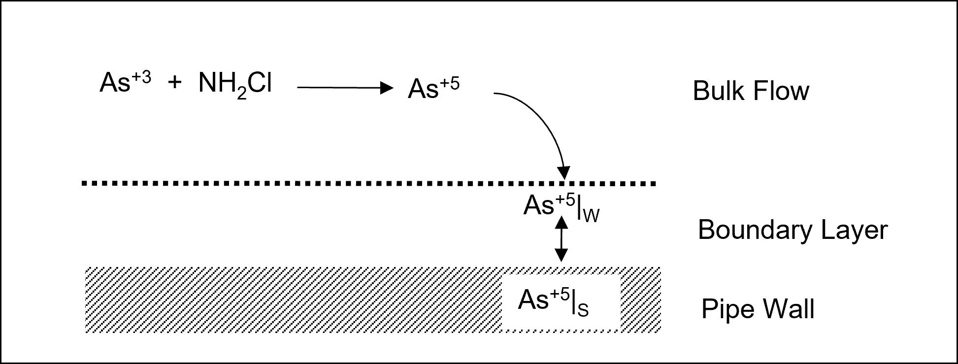
Fig. 5.2 Schematic of the mass transfer limited arsenic oxidation/adsorption system¶

The mathematical form of this reaction system can be modeled with five differential rate equations in the case of non-equilibrium adsorption/desorption (see, e.g., [Gu et al., 1994], for a more complete description of non-equilibrium adsorption/desorption):

(5.5)¶\[\begin{aligned} {d As^{+3} \over {d t}} = -k_a As^{+3}(NH_2Cl) \end{aligned}\]

(5.6)¶\[\begin{aligned} {d (NH_2Cl) \over {d t}} =-k_b (NH_2Cl) \end{aligned}\]

(5.7)¶\[\begin{aligned} {d As^{+5} \over {d t}} = k_a As^{+3}(NH_2Cl)-K_fA_v(As^{+5}-As_w^{+5}) \end{aligned}\]

(5.8)¶\[\begin{aligned} {d As_w^{+5} \over {d t}}= K_fA_v(As^{+5}-As_w^{+5})-A_v[k_1(S_{max}-As_s^{+5})As_w^{+5}-k_2As_s^{+5}] \end{aligned}\]

(5.9)¶\[\begin{aligned} {d As_s^{+5} \over {d t}}= {k_1(S_{max}-As_s^{+5})As_w^{+5}-k_2As_s^{+5}} \end{aligned}\]

where \(As^{+3}\) is the bulk phase concentration of arsenite, \(As^{+5}\) is the bulk phase concentration of arsenate, \(As_w^{+5}\) is the bulk phase concentration of arsenate adjacent to the pipe wall, \(As_s^{+5}\) is surface phase concentration of arsenate, and \(NH_2Cl\) is the bulk phase concentration of monochloramine. The parameters in these equations are as follows: \(k_a\) is a rate coefficient for arsenite oxidation, \(k_b\) is a monochloramine decay rate coefficient due to reactions with all other reactants (including arsenite), \(A_v\) is the pipe surface area per liter of pipe volume, \(k_1\) and \(k_2\) are the arsenate adsorption and desorption rate coefficients, \(S_{max}\) is the maximum pipe surface concentration, and \(K_f\) is a mass transfer rate coefficient. The mass transfer coefficient \(K_f\) will in general depend on the amount of flow turbulence as well as the diameter of the pipe. A typical empirical relation might be:

(5.10)¶\[\begin{aligned} K_f = {{6.67 \times 10^{-6}Re^{0.88}} \over {D}} \end{aligned}\]

where \(Re\) is the flow Reynolds number and \(D\) is the pipe diameter.

Using the notation defined in (2.1)-(2.3), \(\boldsymbol{x}_b\) = {\(As^{+3}\), \(As^{+5}\), \(As_w^{+5}\), \(NH_2Cl\)}, \(\boldsymbol{x}_s\) = {\(As_s^{+5}\)}, \(\boldsymbol{z}_b\) = {\(\emptyset\)}, \(\boldsymbol{z}_s\) = {\(\emptyset\)}, and \(\boldsymbol{p}\) = {\(k_a\), \(k_b\), \(A_v\), \(k_1\), \(k_2\), \(K_f\), \(S_{max}\)}. The reaction dynamics defined by (5.5)-(5.9) conserves total arsenic mass within any pipe segment of length L (and thus bulk volume \(A \times L\), and pipe surface area \(P \times L\), where \(A\) and \(P\) are cross sectional area and wetted perimeter, respectively). This can be shown by summing the differential changes in the mass of all arsenic species within a pipe segment, and assuring that they sum to zero: \((A \times L) ({d {As^{+3}} \over {dt}}) + (A \times L) ({d As^{+5} \over dt}) + (A \times L)({d As_w^{+5} \over dt}) + (P \times L) ({d As_s^{+5} \over dt}) = 0\).

It was mentioned in CONCEPTUAL FRAMEWORK (Section 2) that some reactions are reversible and fast enough in comparison with the system’s other processes so that a local equilibrium can be assumed, while others are not sufficiently fast and/or irreversible and it is inappropriate to use an equilibrium formulation to represent them. In the case of reversible sorption processes a local equilibrium assumption (LEA) is sometimes assumed between the adsorbed phase and its concentration in the bulk fluid (such an assumption is not always realistic, and no such claim is made here - see, e.g., [Koopman et al., 1992]). Under the LEA, the rates of adsorption and desorption must be much faster than the rate of change of the bulk species, and consequently, \({d As_s^{+5} \over dt} = 0\); the differential equation (5.9) can then be substituted with the algebraic equation:

(5.11)¶\[\begin{aligned} As_s^{+5}={{k_s S_{max}As_w^{+5}} \over {1+k_sAs_w^{+5}}} \end{aligned}\]

where \(k_s = k_1/k_2\). In this case the DAE system is described by (5.5)-(5.8) and (5.11), and includes four differential rate equations and one algebraic equation. Thus in terms of the notation used in (2.1)-(2.3), \(\boldsymbol{x}_b\) = {\(As^{+3}\), \(As^{+5}\), \(As_w^{+5}\), \(NH_2Cl\)}, \(\boldsymbol{x}_s\) = {\(\emptyset\)}, \(\boldsymbol{z}_b\) = {\(\emptyset\)}, \(\boldsymbol{z}_s\) = {\(As_s^{+5}\)}, and \(\boldsymbol{p}\) = {\(k_a\), \(k_b\), \(A_v\), \(k_1\), \(k_2\), \(K_f\), \(S_{max}\)}. The LEA model could be left in this form that explicitly includes the surface adsorbed phase (\(As_s^{+5}\)) - or, because the special form of (5.11) presents an explicit solution for the adsorbed arsenate, (5.11) could be substituted into (5.8), leaving an equivalent system of only four differential rate expressions in the four bulk-phase variables \(\boldsymbol{x}_b\) = {\(As^{+3}\), \(As^{+5}\), \(As_w^{+5}\), \(NH_2Cl\)}. In this latter case, however, the adsorbed phase arsenate concentration would have to be separately calculated after solution (if desired), using (5.11), which could be laborious if it were required at many locations and time steps.

Listing 5.3 shows the MSX input file for this system, with the assumption of local equilibrium ((5.5)-(5.8) and (5.11)). The [PIPES] section contains four kinetic rate reactions involving the four bulk species and one equilibrium reaction that includes the lone surface species. The [TANKS] section contains only the bulk species reactions. To complete the model specification, the [QUALITY] section assumes that the network has a single source which is a reservoir node labeled “1”, and that the concentrations at this source remain constant. If this were not the case then a [SOURCES] section could be added that describes the sources in more detail.

Listing 5.3 MSX input file for the mass transfer limited arsenic oxidation/adsorption system¶

[OPTIONS]
  AREA_UNITS  FT2
  RATE_UNITS  HR
  SOLVER      RK5
  TIMESTEP    180

[SPECIES]
  BULK  A3    UG                    ;Dissolved arsenite
  BULK  A5    UG                    ;Dissolved arsenate
  BULK  A5w   UG                    ;Dissolved arsenate at wall
  WALL  A5s   UG                    ;Adsorbed arsenate
  BULK  NH2CL MG                    ;Monochloramine

[COEFFICIENTS]
  CONSTANT  Ka   10.0               ;Arsenite oxidation rate coeff.
  CONSTANT  Kb   0.50               ;Monochloramine decay rate coeff.
  CONSTANT  Smax 50                 ;Arsenate adsorption coeff.  
  CONSTANT  K1   5.0                ;Arsenate adsorption rate coeff.
  CONSTANT  K2   1.0                ;Arsenate desorption rate coeff.

[TERMS]
  Kf     6.67e-4*Re^0.88/D           ;Mass transfer coefficient (Ft/Hr)
  Ks     K1/K2                      ;Arsenate equil. adsorption coeff.
  LPERCF 28.316                     ;Liters/Cu. Ft. (conversion for Kf)

[PIPES]
  RATE  A3    -Ka*A3*NH2CL                        ;Arsenite oxidation                                         
                                                  ;Arsenate production      
  RATE  A5    Ka*A3*NH2CL - LPERCF*Kf*Av*(A5 - A5w)                                        
                                                  ;Arsenate at pipe wall
  RATE  A5w   LPERCF*Kf*Av*(A5 - A5w) - Av*(K1*(Smax-A5s)*A5w - K2*A5s)      
  RATE  NH2CL -Kb*NH2CL                           ;Monochloramine oxidatio                                               
  EQUIL A5s   Smax*Ks*A5w/(1.0 + Ks*A5w) - A5s    ;Arsenate adsorption

[TANKS]
  RATE  A3   -Ka*A3*NH2CL                   ;Arsenite oxidation
  RATE  A5    Ka*A3*NH2CL                   ;Arsenate w/o mass tran.
  RATE  A5w   0                             ;Not present in a tank
  RATE  NH2CL -Kb*NH2CL                     ;Monochloramine oxidation

[QUALITY]
  ;Initial conditions (= 0 if not specified here)
  NODE   1      A3   10.0 
  NODE   1      A5   0.0
  NODE   1      NHCL 2.5

Note about equation units. The modeler must understand the units of all quantities used in mathematical expressions, and ensure that the resulting expressions are dimensionally correct. In short, a complete unit analysis for each expression and resulting RATE or EQUIL term is an essential quality assurance step for developing MSX models. As an example, consider (5.8) above, repeated here for convenience:

\[\begin{aligned} {d As_w^{+5} \over {d t}}= K_fA_v(As^{+5}-As_w^{+5})-A_v[k_1(S_{max}-As_s^{+5})As_w^{+5}-k_2As_s^{+5}] \end{aligned}\]

The units of the left hand side are the units of the bulk species, \(As_w^{+5}\), divided by the units used for time. Since the default time unit is hours, the left hand side has units of [\(\mu g/L\mbox{-}hr\)], and consequently each of the two main terms on the right hand side must have these same units. Since \(A_v\) was previously defined as the pipe surface area per liter pipe volume, and the default area unit is [\(ft^2\)], this quantity has units of [\(ft^2/L\)] (\(A_v\) is a pre-defined MSX hydraulic variable - see the description of the [TERMS] input in INPUT FILE FORMAT (Section 4) of this manual). From this analysis we find that the mass transfer coefficient \(K_f\) in the first term on the right hand side must have units of [\(L/ft^2\mbox{-}hr\)]. The units of the previous expression for \(K_f\) in (5.10) are, however, the more conventional velocity units of [\(ft/hr\)], requiring multiplication by the number of liters per cubic ft: \([ft/hr] \times [L/ ft^3]\) = \([L/ft^2\mbox{-}hr]\). This unit analysis explains the presence of the term LPERCF in the above MSX input file; without this term the expressions would not be dimensionally consistent and the results would be invalid. The reader should verify that the second term on the right hand side is dimensionally correct - given the units of \(A_v\)- provided that rate coefficient \(k_1\) has units [\(L/\mu g\mbox{-}hr\)], and \(k_2\) has units [\(1/hr\)] (recall that the surface species has units of [\(\mu g/ft^2\)], since we are using the default area units).

5.4. Bacterial Regrowth with Chlorine Inhibition¶

This next example models bacterial regrowth as affected by chlorine inhibition within a distribution system. The regrowth model is taken from Zhang et al. [2004] and includes the following processes depicted in Fig. 5.3:

Fig. 5.3 Conceptual diagram of bacterial regrowth within a pipeline. Dashed arrows represent reactions with chlorine while solid arrows represent transformation processes¶

Both free bacteria in the bulk flow and bacteria attached to the pipe wall utilize the biodegradable fraction of dissolved organic carbon (BDOC and DOC, respectively) as a growth substrate. Monod kinetics are used to describe this growth with the following rate equations:

\[ \begin{align}\begin{aligned}\begin{aligned} {{d X}\over {dt}}\bigg |_{growth} = \mu X \end{aligned}\\\begin{aligned} {{d S}\over {dt}} = -\mu X/Y \end{aligned}\end{aligned}\end{align} \]

where \(X\) is mass concentration of bacterial cells, \(S\) is the concentration of BDOC, \(Y\) is a yield coefficient (mass of cells produced per unit conversion of BDOC), and \(\mu\) is a specific growth coefficient. The latter decreases with the BDOC concentration according to:

\[\begin{aligned} \mu = {{\mu_{max}S}\over{S+K_s}} \end{aligned}\]

where \(\mu_{max}\) is the maximum growth rate coefficient and \(K_s\) is the half-saturation constant.

Both free and attached bacteria die at a first order rate:

\[\begin{aligned} {{d X}\over {dt}}\bigg |_{decay} = -k_d X \end{aligned}\]

where \(k_d\) is a decay rate coefficient.

Deposition of free bacterial cells onto the pipe wall is modeled with the following first-order rate process:

\[\begin{aligned} {{d X}\over {dt}}\bigg |_{deposition} = -k_{dep} X \end{aligned}\]

while detachment of attached cells into the bulk flow also depends on flow velocity:

\[\begin{aligned} {{d X}\over {dt}}\bigg |_{detachment} = k_{det} X U \end{aligned}\]

where \(k_{dep}\) is a deposition rate constant, \(k_{det}\) is a detachment rate constant, and \(U\) is the bulk flow velocity.

The effect of chlorine on limiting the number of viable bacterial cells is modeled by applying an inhibition factor \(I\) to the bacterial specific growth rate as:

\[\begin{aligned} I = exp \left ( {-(C-C_t)}\over {C_c}\right) \end{aligned}\]

Here \(C\) is the chlorine concentration, \(C_t\) is a threshold chlorine concentration below which no inhibition occurs, and \(C_c\) is a characteristic chlorine concentration that scales the degree of inhibition. Note at higher values of \(C\), \(I\) becomes smaller and therefore results in smaller bacterial growth rates.

Chlorine reacts with DOC in the bulk flow to decay at a first-order rate:

\[\begin{aligned} {{d C}\over {dt}} = -k_{b} C \end{aligned}\]

where \(C\) is chlorine concentration and \(k_b\) is a bulk decay rate coefficient.

The EPANET-MSX specification of the full model is shown in Figure Listing 5.4.

Listing 5.4 MSX input file for a bacterial regrowth model with chlorine inhibition¶

[OPTIONS]
AREA_UNITS  CM2
RATE_UNITS  HR
SOLVER      RK5
TIMESTEP    300

[SPECIES]
BULK   CL2   MG          ;chlorine
BULK   S     MG          ;organic substrate
BULK   Xb    UG          ;mass of free bacteria
WALL   Xa    UG          ;mass of attached bacteria
BULK   Nb    log(N)      ;number of free bacteria
WALL   Na    log(N)      ;number of attached bacteria

[COEFFICIENTS]
CONSTANT  Kb      0.05   ;CL2 decay constant (1/hr)
CONSTANT  CL2C    0.20   ;characteristic CL2 (mg/L)
CONSTANT  CL2Tb   0.03   ;threshold CL2 for Xb (mg/L)
CONSTANT  CL2Ta   0.10   ;threshold CL2 for Xa (mg/L)
CONSTANT  MUMAXb  0.20   ;max. growth rate for Xb (1/hr)
CONSTANT  MUMAXa  0.20   ;max. growth rate for Xa (1/hr)
CONSTANT  Ks      0.40   ;half saturation constant (mg/L)
CONSTANT  Kdet    0.03   ;detachment rate constant (1/hr/(ft/s))
CONSTANT  Kdep    0.08   ;deposition rate constant (1/hr)
CONSTANT  Kd      0.06   ;bacterial decay constant (1/hr)
CONSTANT  Yg      0.15   ;bacterial yield coefficient (mg/mg)

[TERMS]
Ib   EXP(-STEP(CL2-CL2Tb)*(CL2-CL2Tb)/CL2C) ;Xb inhibition coeff. 
Ia   EXP(-STEP(CL2-CL2Ta)*(CL2-CL2Ta)/CL2C) ;Xa inhibition coeff.
MUb  MUMAXb*S/(S+Ks)*Ib                     ;Xb growth rate coeff.
MUa  MUMAXa*S/(S+Ks)*Ia                     ;Xa growth rate coeff.

[PIPES]
RATE    CL2    -Kb*CL2
RATE    S      -(MUa*Xa*Av + MUb*Xb)/Yg/1000
RATE    Xb     (MUb-Kd)*Xb + Kdet*Xa*U*Av - Kdep*Xb
RATE    Xa     (MUa-Kd)*Xa - Kdet*Xa*U + Kdep*Xb/Av
FORMULA Nb     LOG10(1.0e6*Xb)
FORMULA Na     LOG10(1.0e6*Xa)

[TANKS]
RATE    CL2    -Kb*CL2
RATE    S      -MUb*Xb/Yg/1000
RATE    Xb     (MUb-Kd)*Xb
FORMULA Nb     LOG10(1.0e6*Xb)

[SOURCES]
CONCEN  SrcNode  CL2  1.2
CONCEN  SrcNode  S    0.4
CONCEN  SrcNode  Xb   0.01

Several notes of explanation require mentioning:

There are six species defined for the model: bulk chlorine (CL2), bulk biodegradable dissolved organic carbon (S), bulk bacterial concentration (Xb), bulk bacterial cell count (Nb), attached bacterial concentration (Xa), and attached bacterial cell count (Na). CL2 and S are measured in milligrams. The bacterial concentrations are expressed in micrograms of equivalent carbon so that their numerical values scale more evenly. The bacterial cell counts are expressed as the logarithm of the number of cells.
The entries in the [PARAMETERS] section are based on values provided by Zhang et al. [2004] and are used only for illustrative purposes.
The [TERMS] section allows one to define intermediate mathematical terms in the model’s description so that the rate equations can be expressed more clearly and compactly.
The chlorine inhibition threshold concentration is lower for the bulk phase than for the surface phase. This results in defining separate inhibition factors, Ib and Ia for these two phases, respectively.
The special EPANET-MSX function STEP(x) used in the definitions of the inhibition factors Ib and Ia is internally evaluated to 1 when x > 0 and is 0 otherwise.
The variables U and Av are reserved symbols (see Section 4.5) in EPANET-MSX that represent flow velocity and pipe surface area per unit volume, respectively, and their values are automatically computed by the program.
Whenever the surface biomass species appears in the rate expression for a bulk species it is multiplied by Av to convert from areal density to volumetric concentration. Likewise, the bulk biomass concentration is divided by Av in the rate expression for attached biomass to convert it to an areal density.
The kinetic rate expressions for tanks do not include any terms involving Xa since it is assumed that surface species do not exist (or have reduced significance) within storage facilities.
A simple FORMULA expression is used to convert from micrograms of bacterial carbon to logarithmic cell counts. It assumes that there are \(10^6\) cells per microgram of carbon in the cell biomass.
The model assumes that there is a single source node named SrcNode that supplies all water to the system. The [SOURCES] section specifies the concentrations of chlorine, biodegradable carbon, and bulk bacterial concentration in this water. The latter value was derived from assuming that the treated source water contained 10 cells/mL (i.e., \(10^4\) cells per liter).

5.5. Chloramine Decomposition¶

This final example illustrates a complex chemical reaction system involving both kinetic rate expressions and nonlinear equilibrium relationships. The system being studied is the auto-decomposition of monochloramine to ammonia in the presence of natural organic matter (NOM). When chloramines are used as a secondary disinfectant care must be taken to avoid producing excessive amounts of free ammonia that can contribute to biological nitrification episodes within the distribution system. The reaction model used for this system was developed by Valentine and co-workers [Duirk et al., 2005, Vikesland et al., 2001] and is shown in Table Table 5.1. The principal species are hypochlorous acid (HOCl), hypochlorite ion (OCL^-), ammonia (NH₃), ammonium ion (NH₄⁺), monochloramine (NH₂Cl), dichloramine (NHCl₂), an unidentified intermediate compound (I), and total organic carbon (TOC). Because the reactions involve acid-base dissociations and the rate coefficient of the disproportionation of NH₂Cl is a function of both pH and carbonate species, the pH-carbonate equilibrium system is also included.

Listing 5.5 shows the EPANET-MSX specification of the monochloramine decay model. There are 14 bulk species and no surface species. The entries in the [COEFFICIENTS] section are the rate coefficients \(k_1\) through \(k_{12}\) listed in Table 5.1. The expression for \(k_5\) as a function of pH and carbonate species is included in the [TERMS] section, as are the rate terms contributed by the reactants of reactions 1 through 12 in Table 5.1. Because there are no surface species in the model, the reaction expressions listed in the [PIPES] section apply to the storage tanks as well.

The first five rate expressions apply to the various chlorinated species, ammonia, and the un-named intermediate compound. The next three rate expressions, all set equal to 0, state that pH, alkalinity, and TOC are assumed to remain constant. These are followed by two equilibrium expressions that represent the dissociation reactions of hypochlorous acid and ammonia, respectively. The final set of four equilibrium expressions model the distribution of the various carbonate species under conditions of constant alkalinity and pH. Note that in order to solve this carbonate equilibrium sub-system it is necessary to supply initial values for pH and alkalinity at all nodes of whatever network is being modeled. This is done in the [QUALITY] section, using the GLOBAL specifier to set values throughout the network. (The alkalinity of 0.004 moles/L is equivalent to 200 \(mg/L\) CaCO₃ while the H⁺ value of \(2.818 \times 10^{-8}\) moles/L is the same as a pH of 7.55.)

Table 5.1 Monochloramine decay model based on Vikesland et al. (2001) and Duirk et al. (2005).¶
	Reaction Stoichiometry	Rate Coefficient/Equilibrium Constant^a
R.1	HOCl + NH₃ \(\rightarrow\) NH₂Cl + H₂O	\(k_1=1.5 \times 10^{10} M^{-1}h^{-1}\)
R.2	NH₂Cl + H₂O \(\rightarrow\) HOCl + NH₃	\(k_2=7.6 \times 10^{-2}\,h^{-1}\)
R.3	HOCl + NH₂Cl \(\rightarrow\) NHCl₂ + H₂O	\(k_3=1.0 \times 10^{6}M^{-1}\,h^{-1}\)
R.4	NHCl₂ + H₂O \(\rightarrow\) HOCl + NH₂Cl	\(k_4=2.3 \times 10^{-3}\,h^{-1}\)
R.5	NH₂Cl + NH₂Cl \(\rightarrow\) NHCl₂ + NH₃	\(k_5=2.5 \times 10^{7}[H^{+}]+4.0 \times 10^{4}[H_2CO_3] +800[HCO_3^{-}]\,M^{-2}h^{-1}\)
R.6	NHCl₂ + NH₃ \(\rightarrow\) NH₂Cl + NH₂Cl	\(k_6=2.2 \times 10^{8}\,M^{-2}h^{-1}\)
R.7	NHCl₂ + H₂O \(\rightarrow\) I	\(k_7=4.0 \times 10^{5}\,M^{-1}h^{-1}\)
R.8	I + NHCl₂ \(\rightarrow\) HOCl + products	\(k_8=1.0 \times 10^{8}\,M^{-1}h^{-1}\)
R.9	I + NH₂Cl \(\rightarrow\) products	\(k_9=3.0 \times 10^{7}\,M^{-1}h^{-1}\)
R.10	NH₂Cl + NHCl₂ \(\rightarrow\) products	\(k_{10}=55.0\,M^{-1}h^{-1}\)
R.11	NH2Cl + S₁\(\times\) TOC \(\rightarrow\) products^b	\(k_{11}=3.0 \times 10^{4}\,M^{-1}h^{-1}\) \(S_1\) = 0.02
R.12	HOCl + S₂\(\times\) TOC \(\rightarrow\) products^c	\(k_{12}=6.5 \times 10^{5}\,M^{-1}h^{-1}\) \(S_2\) = 0.5

E.1	HOCl \(\leftrightarrow\) H⁺ + OCl^-	\(pK_a\) = 7.5
E.2	NH₄⁺ \(\leftrightarrow\) NH₃ + H⁺	\(pK_a\) = 9.3
E.3	H₂CO₃ \(\leftrightarrow\) HCO₃^- + H⁺	\(pK_a\) = 6.3
E.4	HCO₃^- \(\leftrightarrow\) CO₃^2- + H⁺	\(pK_a\) = 10.3

\(\ \ \ \ \) Notes:

All rate coefficients and equilibrium constants are for 25 degrees C.

\(S_1\) is the fast reactive fraction of TOC.

\(S_2\) is the slow reactive fraction of TOC.

Listing 5.5 EPANET-MSX input file of the monochloramine decomposition model¶

[OPTIONS]
RATE_UNITS  HR
SOLVER      ROS2
COUPLING    NONE
TIMESTEP    300
RTOL        0.0001
ATOL        1.0e-8

[SPECIES]
BULK   HOCL    MOLES    ;hypochlorous acid
BULK   NH3     MOLES    ;ammonia
BULK   NH2CL   MOLES    ;monochloramine
BULK   NHCL2   MOLES    ;dichloramine
BULK   I       MOLES    ;unknown intermediate
BULK   OCL     MOLES    ;hypochlorite ion
BULK   NH4     MOLES    ;ammonium ion
BULK   ALK     MOLES    ;total alkalinity
BULK   TOC     MOLES    ;total organic carbon
BULK   H       MOLES    ;hydrogen ion
BULK   OH      MOLES    ;hydroxide ion
BULK   CO3     MOLES    ;carbonate ion
BULK   HCO3    MOLES    ;bicarbonate ion
BULK   H2CO3   MOLES    ;dissolved carbon dioxide

[COEFFICIENTS]
PARAMETER       k1    1.5e10
PARAMETER       k2    7.6e-2
PARAMETER       k3    1.0e6
PARAMETER       k4    2.3e-3
PARAMETER       k6    2.2e8
PARAMETER       k7    4.0e5
PARAMETER       k8    1.0e8
PARAMETER       k9    3.0e7
PARAMETER       k10   55.0

PARAMETER       k11   3.0E4
PARAMETER       k12   6.5E5
CONSTANT        S1    0.02
CONSTANT        S2    0.50

[TERMS]
k5     (2.5e7*H) + (4.0e4*H2CO3) + (800*HCO3)
a1     k1*HOCL*NH3
a2     k2*NH2CL
a3     k3*HOCL*NH2CL
a4     k4*NHCL2
a5     k5*NH2CL*NH2CL
a6     k6*NHCL2*NH3*H
a7     k7*NHCL2*OH
a8     k8*I*NHCL2
a9     k9*I*NH2CL
a10    k10*NH2CL*NHCL2
a11    k11*S1*TOC*NH2CL
a12    k12*S2*TOC*HOCL

[PIPES]
RATE   HOCL    -a1 + a2 - a3 + a4 + a8 – a12
RATE   NH3     -a1 + a2 + a5 - a6 + a11
RATE   NH2CL    a1 - a2 - a3 + a4 - a5 + a6 - a9 - a10 – a11
RATE   NHCL2    a3 - a4 + a5 - a6 - a7 - a8 - a10
RATE   I        a7 - a8 - a9
RATE   H        0
RATE   ALK      0
RATE   TOC      0
EQUIL  OCL      H*OCL - 3.16E-8*HOCL
EQUIL  NH4      H*NH3 - 5.01E-10*NH4
EQUIL  CO3      H*CO3 - 5.01E-11*HCO3
EQUIL  H2CO3    H*HCO3 - 5.01E-7*H2CO3
EQUIL  HCO3     ALK - HCO3 - 2*CO3 - OH + H
EQUIL  OH       H*OH - 1.0E-14

[QUALITY]
GLOBAL       ALK   0.004
GLOBAL       H     2.818E-8