2. CONCEPTUAL FRAMEWORK
From a water quality modeling perspective, two significant physical phases exist within a water distribution system: a mobile bulk water phase and a fixed pipe surface phase. Bulk phase species are chemical or biological components that exist within the bulk water phase and are transported through the system with the average water velocity. Surface phase species are components that are attached or incorporated into the pipe wall and are thus rendered immobile. Fig. 2.1 shows an example of bulk phase chlorine (HOCl) reacting with bulk phase NOM (natural organic matter) to produce a bulk phase disinfectant by-product (DBP), while also oxidizing ferrous iron to ferric iron in the fixed surface phase at the pipe wall.
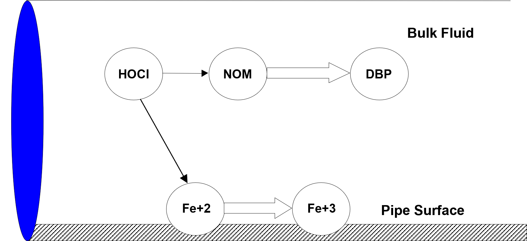
Fig. 2.1 Example of reactions in the mobile bulk phase and at the fixed pipe surface phase.
Examples of bulk species include dissolved constituents (individual compounds or ions, such as HOCl and OCl-, as well as aggregate components such as TOC), suspended constituents (such as bacterial cells and inorganic particulates), and chemicals adsorbed onto particles. Examples of surface species include bacteria incorporated within biofilm, oxidized forms of iron contained within corrosion scale, particulate material that settles out due to gravity or is attached to the pipe wall surface through ionic or molecular (i.e., van der Waal) forces, and organic compounds that can diffuse into or out of plastic pipes or be adsorbed onto or desorbed from iron oxide pipe surfaces. Some components, such as bacteria and particulates, can exist in both the bulk and surface phases and transfer from one phase to another by such mechanisms as physical attachment/detachment, chemical adsorption or molecular diffusion. In such situations, the component is modeled as two species: one bulk and the other surface.
Additional phases that might exist within a distribution system, such as a mobile bed sediment phase, an immobile water phase within the pore structure of pipe scale, or an air phase overlying the water surface in a storage tank, could also be included within this modeling framework.
2.1. Material Transport
A water distribution system consists of pipes, pumps, valves, fittings, and storage facilities that convey water from source points to consumers. This physical system is modeled as a network of links connected together at nodes in some particular branched or looped arrangement. Fig. 2.2 provides an example of a network representation of a very simple distribution system. Links represent pipes, pumps, and valves; nodes serve as source points, consumption points and storage facilities. The following phenomena all influence the quality of water contained in the system and can be modeled using principles of conservation of mass coupled with reaction kinetics:
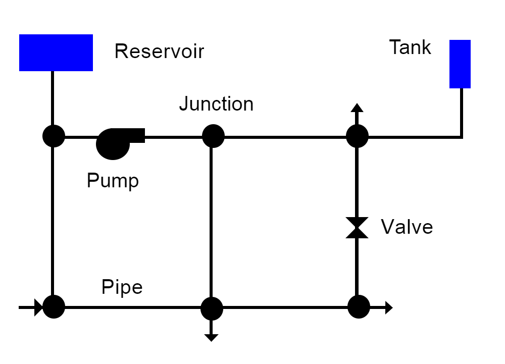
Fig. 2.2 Node-link representation of a simple distribution system.
Advective transport in pipes: bulk species are transported down the length of a pipe with the same average velocity as the carrier fluid while at the same time reacting with other bulk species and with the pipe wall surface.
Dispersive transport in pipes: due to the differences of concentration and the distribution of the radial flow velocity, bulk species spread from highly concentrated to less concentrated areas.
Mixing at pipe junctions: at junctions receiving inflow from two or more links the flows are assumed to undergo complete and instantaneous mixing.
Mixing in storage nodes: all inflows to storage nodes mix completely with the existing contents in storage while these contents are subjected to possible bulk phase reactions (alternative schemes are available for modeling plug flow storage tanks).
2.2. Chemical Reactions
Reactions can be divided into two classes based on reaction rates. Some reactions are reversible and fast enough in comparison with the system’s other processes so that a local equilibrium can be assumed; others are not sufficiently fast and/or irreversible and it is inappropriate to use an equilibrium formulation to represent them. Theoretically, very large backward and forward rate constants (with their ratio equaling the equilibrium constant) can be used to model fast/equilibrium reactions and therefore both fast/equilibrium and slow/kinetic reaction dynamics can be written as a single set of ordinary differential equations (ODEs) that can be integrated over time to simulate changes in species concentrations. This approach can result in reaction rates that may range over several orders of magnitude and lead to such small integration time steps so as to make a numerical solution impractical.
In EPANET-MSX, algebraic equations are used to represent the fast/equilibrium reactions and mass conservation. Thus it is assumed that all reaction dynamics can be described by a set of differential-algebraic equations (DAEs) in semi-explicit form. The system of DAEs that defines the interactions between bulk species, surface species, and parameter values can be written in general terms as:
(2.1)¶\[\begin{aligned} \frac{d \boldsymbol{x_b}} {d {t}} = \boldsymbol {f(x_b, x_s, z_b, z_s, p)} \end{aligned}\](2.2)¶\[\begin{aligned} \frac{d\boldsymbol{x_s}} {d {t}}= \boldsymbol {g(x_b, x_s, z_b, z_s, p)} \end{aligned}\](2.3)¶\[\begin{aligned} \boldsymbol{0} = \boldsymbol{h(x_b, x_s, z_b, z_s, p)} \end{aligned}\]
where the vectors of time-varying differential variables \(\boldsymbol{x_b}\) and \(\boldsymbol{x_s}\) are associated with the bulk water and pipe surface, respectively, the time-varying algebraic variables \(\boldsymbol{z_b}\) and \(\boldsymbol{z_s}\) are similarly associated, and the model parameters \(\boldsymbol{p}\) are time invariant. The algebraic variables are assumed to reach equilibrium in the system within a much smaller time scale compared to the numerical time step used to integrate the ODEs. The dimension of the algebraic equations \(\boldsymbol{h}\) must agree with that of the algebraic variables \(\boldsymbol{z}\) = [\(\boldsymbol{z_b}\) \(\boldsymbol{z_s}\)], so that the total number of equations in (2.1)-(2.3) equals the total number of time-varying species ([\(\boldsymbol{x_b}\) \(\boldsymbol{x_s}\) \(\boldsymbol{z_b}\) \(\boldsymbol{z_s}\)]).
As a simple example of a reaction/equilibrium system modeled as a set of DAEs, consider the oxidation of arsenite (\(As^{+3}\)) to arsenate (\(As^{+5}\)) by a monochloramine disinfectant residual in the bulk flow and the subsequent adsorption of arsenate onto exposed iron on the pipe wall. (Arsenite adsorption is not significant at the pH’s typically found in drinking water.) A more complete explanation and extension of this model is presented in EXAMPLE REACTION SYSTEMS (Section 5) of this manual. This system consists of four species (arsenite, arsenate, and monochloramine in the bulk flow, and sorbed arsenate on the pipe surface). It can be modeled with three differential rate equations and one equilibrium equation:
where \(As^{+3}\) is the bulk phase concentration of arsenite, \(As^{+5}\) is the bulk phase concentration of arsenate, \(As_s^{+5}\) is surface phase concentration of arsenate, and \(NH_2Cl\) is the bulk phase concentration of monochloramine. The parameters in these equations are as follows: \(k_a\) is a rate coefficient for arsenite oxidation, \(k_b\) is a monochloramine decay rate coefficient, \(A_v\) is the pipe surface area per liter pipe volume, \(k_1\) and \(k_2\) are arsenate adsorption and desorption rate coefficients, \(S_{max}\) is the maximum pipe surface concentration of arsenate, and \(k_s\) = \(k_1/k_2\). Thus in terms of the notation used in (2.1)-(2.3), \(\boldsymbol{x_b} = {\{As^{+3}, As^{+5}, NH_2Cl\}}\), \(\boldsymbol{x_s} = {\{\emptyset\}}\), \(\boldsymbol{z_b} = {\{\emptyset\}}\), \(\boldsymbol{z_s} = {\{As_s^{+5}\}}\), \(\boldsymbol{p} = {\{k_a, k_b, A_v, k_1, k_2, S_{max}\}}\). Example input files for this form of the model are included with the standard EPANET-MSX distribution, while the input file for a more complex version of the model is presented in EXAMPLE REACTION SYSTEMS (Section 5).
2.3. Full Network Solution
Dynamic models of water quality within water distribution systems can be classified spatially as either Eulerian or Lagrangian. Eulerian models divide the network into a series of fixed control elements and record the changes at the boundaries and within these elements, while Lagrangian models track changes of discrete parcels of water as they travel through the network. EPANET-MSX utilizes the Lagrangian transport algorithm as used by EPANET. It tracks the movement and reaction of chemicals in discrete water volumes, or segments. These segments are transported through network pipes by the bulk velocity, and completely mix at junction nodes. This method is relatively efficient because the number and size of the segments in a pipe can change as hydraulic conditions change. In addition, EPANET-MSX adds the effect of longitudinal dispersion to EPANET’s Lagrangian transport algorithm.The details of the Lagranigain algorithm to model advection, dispersion and reaction are described in [Shang et al., 2021].
In summary form, the following steps, depicted visually in Fig. 2.3, are performed for each water quality time step:
React: Apply reaction dynamics within each pipe segment and storage tank over the time step to compute new concentrations throughout the network.
Advect: Within each pipe, compute the flow volume transported over the time step and transfer this amount of volume and its associated bulk species mass from the pipe’s leading segments into accumulated mass and volume totals at the downstream node.
Mix: Compute new bulk species concentrations at each node based on its accumulated mass and volume inputs from the advection step as well as any external sources.
Release: Create a new segment at the upstream end of each pipe whose size equals the pipe’s flow volume and whose bulk species concentrations equal that of the upstream node (or if the difference in quality between the most upstream segment and the upstream node is below some tolerance, simply increase the size of the current upstream segment).
Disperse: Solve the disperison process equation and update both nodal and segment concentrations.
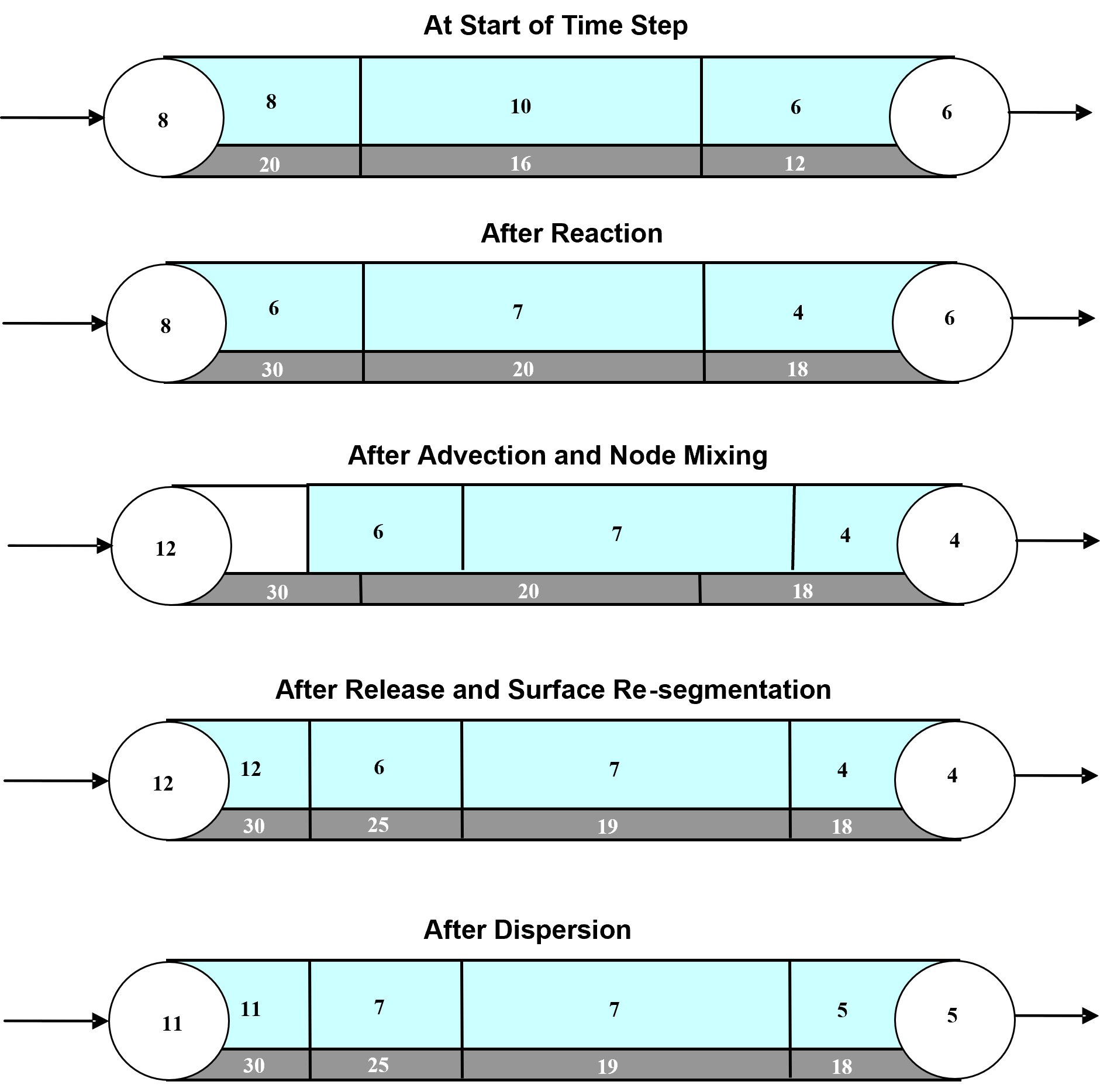
Fig. 2.3 Illustration of the 5-step water quality transport method for pipe networks. The upper pipe segments contain flowing water while the lower segments are the pipe wall surface. The numbers in each segment represent hypothetical bulk and surface species concentrations, respectively.
2.4. Reaction System Solution
The multi-species water quality algorithm modifies the React step (step 1) of the solution scheme described above. Within each pipe segment, reaction dynamics are represented by the system of DAEs (2.1)-(2.3). The same applies for storage tanks, except that the DAEs are modified to consider only bulk reactions. Although not indicated, the model parameters p can possibly vary by pipe. For the equilibrium reactions, it is assumed that the Jacobian matrix of \(\boldsymbol{h}\) with respect to \(\boldsymbol{z}\), \(\partial \boldsymbol{h} \over \partial \boldsymbol{z}\), is unique and nonsingular for all \(t\). In this case, the implicit functions defined by (2.3),
exist, are continuous and unique, and possess continuous partial derivatives. These properties, and in particular the resultant ability to evaluate (2.8)-(2.9) (numerically), are central to the numerical algorithms used for solution of (2.1)-(2.3).
Given the implicit functions (2.8)-(2.9), the solution of (2.1)-(2.3) is performed by substituting (2.8)-(2.9) into (2.1)-(2.2), thus eliminating the algebraic equations (2.3) and leaving a reduced system of ordinary differential equations (ODEs) that can be integrated numerically:
Note that the above “substitution” is not performed literally, since (2.8)-(2.9) are implicit, and thus so are the reduced trajectories \(\boldsymbol{f'}\) and \(\boldsymbol{g'}\). Solving (2.10)-(2.11) numerically with an explicit method, such as any of the Runge-Kutta schemes, will require that \(\boldsymbol{f'}\) and \(\boldsymbol{g'}\) be evaluated at intermediate values of \(\boldsymbol{x_b}\) and \(\boldsymbol{x_s}\) over the integration time step. Each such evaluation will in turn require a solution of the nested set of algebraic equations (2.8)-(2.9). Alternative strategies for accomplishing these steps are discussed in the Model Implementation (Section 2.7) below.
In addition to the React step, evaluation of the equilibrium equations also needs to be performed at the Mix phase of the overall algorithm since the blending together of multiple flow streams can result in a new equilibrium condition. This process needs to be performed at each network node, including storage tanks.
2.5. Pipe Surface Discretization
The segment bulk water state variables \(\boldsymbol{x_b}\) and \(\boldsymbol{z_b}\) have moving coordinates, due to the nature of the Lagrangian water quality model (they move with the bulk water velocity). In contrast the associated pipe surface variables \(\boldsymbol{x_s}\) and \(\boldsymbol{z_s}\) have fixed coordinates, since they are associated with the non-moving pipe. The lack of a common fixed coordinate system for the bulk and surface state variables must be reconciled, since these variables interact through the common pipe-water interface (through equations (2.1)-(2.3)). To resolve this issue a simple mass-conserving scheme is applied at every water quality time step to update the pipe surface elements to remain consistent with the (advected) water quality segments and re-distribute the surface variable mass among the updated elements.
As shown in Fig. 2.3, within any single water quality time step, a moving mesh divides each pipe surface into discrete-length elements, such that each shares a common surface/water interface with the water quality segment above it. At the end of the time step the pipe elements will, however, be inconsistent with the water quality segments, due to advection of the latter (i.e., through the Advect step of the overall algorithm). This inconsistency is removed by updating the surface species concentrations using an interfacial area-weighted average:
where \(i\) is the water quality segment index, \(n\) is the number of water quality segments in the pipe during the most recent React step, \(L_j\) is the length of segment \(j\), with corresponding vectors of surface species \(\boldsymbol{x}_{sj}\) and \(\boldsymbol{z}_{sj}\), \(n^{new}\) is the updated number of water quality segments in the pipe after advection, \(L_i^{new}\) is the length of each updated segment, with corresponding updated surface concentrations \(\boldsymbol{x}_{si}^{new}\) and \(\boldsymbol{z}_{si}^{new}\). The quantity \((L_i^{new} \cap L_j)\) is the length of the overlapping intersection between segment \(j\) and updated segment \(i\).
2.6. Dispersion Modeling
One-dimensional mass transport in a pipe with a uniform cross-sectional area can be described as advection-dispersion-reaction equations. For a specific species,
(2.14)¶\[\begin{aligned} \frac{\partial {c_i}} {\partial {t}} + u \frac{\partial {c_i}} {\partial {x}}= D_i\frac{\partial^2 {c_i}} {\partial {x^2}}+r(\boldsymbol{c}) \end{aligned}\]
where \(i\) = species index; \(c_i\) = concentration of the species \(i\); \(u\) = flow velocity; \(x\) = distance alone the pipe’s longitudinal direction; \(D_i\) = effective dispersion coefficient of the species \(i\); \(r_i\) = reaction rate of the species \(i\); and \(\boldsymbol{c}\) = the concentration vector of all species which includes both differential and algebraic variables as defined in Chemical Reactions (Section 2.2).
The impact of dispersion may be negligible for many parts of water distribution systems under highly turbulent conditions. However, it is important to consider dispersion when modeling dead-end segments of a system or premise plumbing systems where the flow Reynolds number can be low. The relative importance of the dispersion can be quantified with the Peclet number:
(2.15)¶\[\begin{aligned} Pe_i = {\frac{ul} {D_i}} \end{aligned}\]
where \(l\) = pipe length. The Peclet number is a dimensionless measure of the relative importance of advection versus dispersion, where a large number indicates an advection-dominated flow condition in which the dispersion is negligible.
The effective longitudinal dispersion coefficient accounts for the combined effect of molecular diffusion and shear dispersion due to the nonuniformity of the velocity profile. For laminar flow conditions (Reynolds number less than 2300), the effective dispersion coefficient is calcuated as an averaged value over the residence time [Lee, 2004]:
(2.16)¶\[\begin{aligned} D = {\frac {a^2u^2} {48D_m}}\left[1-\left[\frac{1-exp\left(-16\frac{D_mt_r}{a^2}\right)}{16{\frac{D_mt_r}{a^2}}} \right] \right] \end{aligned}\]
where \(D_m\) = molecular diffusion coefficient; \(a\) = pipe radius; and \(t_r\) = pipe residence time (\(\frac {l} {u}\)).
For turbulent and transitional flow conditions, the effective dispersion coefficient does not depend on the molecular diffusion coefficient and the formula used is [Basha and Malaeb, 2007]:
(2.17)¶\[\begin{aligned} D = au_{\ast}\left[10.1+577\left(\frac{Re}{1000}\right)^{-2.2}\right] \end{aligned}\]
where \(u_{\ast}\) = shear velocity; and \(Re\) = the Reynolds number.
2.7. Model Implementation
EPANET-MSX offers several choices of numerical integration methods for solving the reaction system’s ODEs, equations (2.1) and (2.2). These include a forward Euler method (as used in EPANET), a fifth order Runge-Kutta method with automatic time step control [Hairer et al., 1993], and a second order Rosenbrock method with automatic time step control [Verwer et al., 1992]. These are listed in order of the numerical work per time step required to obtain a solution. The Euler method is best applied to non-stiff, linear reaction systems, the Runge-Kutta method to non-stiff, nonlinear systems, and the Rosenbrock method to stiff systems (see, e.g., Golub and Ortega [1992]).
The algebraic equilibrium equations (2.3) are solved using a standard implementation of the Newton method [Press et al., 1992]. This algorithm requires that the Jacobian of \(\boldsymbol{h}\) with respect to the algebraic variables \(\boldsymbol{z_b}\) and \(\boldsymbol{z_s}\) be used to iteratively solve an approximating linear system of equations until convergence is achieved. This can be a computationally expensive procedure since the Jacobian must be evaluated numerically and the system (2.3) is being solved within every pipe segment of every pipe at every time step, possibly several times over, as the ODEs are integrated. To help reduce this burden EPANET-MSX offers the following options for evaluating the nonlinear equilibrium equation system:
The Non-Coupled option only evaluates the equilibrium equations at the end of the time step after a new ODE solution has been found; the algebraic variables maintain the values they had at the start of the time step while the ODEs are being numerically integrated.
The Fully-Coupled option solves the algebraic equations at each stage of the ODE solution process using a fresh Jacobian for each Newton step.
The choice of coupling involves a trade-off between computational effort and level of accuracy, the degree of which will likely be very system dependent.
A mass balance report is provided for all species that are represented by the differential variables, \(\boldsymbol{x_b}\) and \(\boldsymbol{x_s}\). For each species the report lists the ratio of the total mass entering the system to the total mass leaving the system (including mass lost to reaction).
Dispersion modeling of particular species can be excluded from the network solution procedure by not assigning them a molecular diffusivity. It can also be excluded for pipes that experience highly turbulent flow resulting in a Peclet number ((2.15)) above a user-specified limit.