3. PROGRAM USAGE
EPANET-MSX is a 64-bit application that runs under Microsoft Windows 7 or higher. It is distributed in a compressed archive file named EPANETMSX.ZIP. The contents of this archive are listed in Table 3.1. The top level archive folder contains a Readme.txt file that describes the contents of the archive and procedures for reporting bugs.
Readme.txt |
describes the contents of the archive |
\bin
runepanetmsx.exe
epanetmsx.dll
epanet2.dll
vcomp140.dll
runvc.bat
|
command line version of EPANET-MSX
EPANET-MSX function library
standard EPANET function library
Visual Studio C/C++ OpenMP Runtime library
batch file to launch the Visual Studio C/C++ compiler and comiple the reaction equations (see the section Using Compiled Reaction Models)
|
\Examples
example1.inp
example1.msx
example1.rpt
example2.inp
example2.msx
example2.rpt
|
EPANET input file for example 1
MSX input file for example 1
report file containing the MSX results for example 1
EPANET input file for example 2
MSX input file for example 2
report file containing the MSX results for example 2
|
\Doc
epanetmsx.pdf
license.txt
|
EPANET-MSX users manual
licensing agreement for using EPANET-MSX
|
\Include
epanetmsx.h
epanetmsx.bas
epanetmsx.pas
epanet2.h
epanet2_enums.h
epanet2.bas
epanet2.pas
epanetmsx.lib
epanet2.lib
|
C/C++ header file for EPANET-MSX toolkit
Visual Basic declarations of EPANET-MSX functions
Delphi-Pascal declarations of EPANET-MSX functions
C/C++ header file for EPANET2.2 toolkit
C/C++ header file for the symbolic constants used by EPANET2.2 Toolkit
Visual Basic declarations of EPANET2 functions
Delphi-Pascal declarations of EPANET2 functions
Microsoft C/C++ LIB file for epanetmsx.dll
Microsoft C/C++ LIB file for epanet2.dll
|
\Src |
EPANET-MSX source files |
Most end users will only need to extract the files in the \bin, \examples, and \doc folders to a directory of their choosing. Developers will also need the files in the \include folder to write custom applications. They should also be aware of the licensing requirements set forth in the license.txt file.
The EPANET-MSX system is supplied as both:
a stand-alone console application (runepanetmsx.exe) that can run standard water quality analyses without any additional programming effort required,
a function library (epanetmsx.dll) that, when used in conjunction with the original EPANET function library (epanet2.dll), can produce customized programming applications.
At this point in time the extension has not been integrated into the Windows version of EPANET. This is expected to happen at some future date. Examples of each type of usage are provided below.
Regardless of which approach is used, the user must prepare two input files to run a multi-species analysis. One of these is a standard EPANET input file that describes the hydraulic characteristics of the network being analyzed (EPANET-MSX will ignore any water quality information that might be in this file). The format of this file is described in the EPANET Users Manual [Rossman, 2000, Rossman et al., 2020]. Any network file that was created, edited and then exported from the Windows version of EPANET can serve as the EPANET input file for the multi-species extension.
The second file that must be prepared is a special EPANET-MSX file that describes the species being simulated and the chemical reaction/equilibrium model that governs their dynamics. The format of this file is described in INPUT FILE FORMAT (Section 4) of this manual.
3.1. Example Command Line Run
In order to demonstrate the use of the command line version of EPANET-MSX we will simulate the arsenic oxidation/adsorption reaction system that was briefly described in CONCEPTUAL FRAMEWORK (Section 2) of this manual using the simple pipe network shown in Fig. 3.1 that was adapted from Zhang et al. [2004]. Table 3.2 lists the properties associated with the nodes of this network while Table 3.3 does the same for the pipe links.
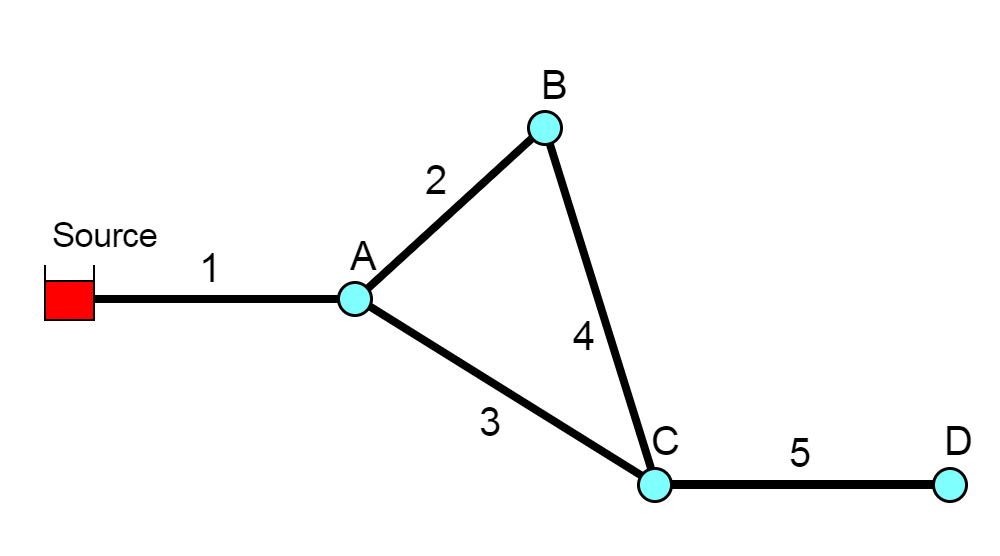
Fig. 3.1 Schematic of the example pipe network
Node |
Elevation (\(m\)) |
Demand (\(m^3/hr\)) |
|---|---|---|
Source |
100 |
– |
A |
0 |
4.1 |
B |
0 |
3.4 |
C |
0 |
5.5 |
D |
0 |
2.3 |
Pipe |
Length (\(m\)) |
Diameter (\(mm\)) |
C-Factor |
|---|---|---|---|
1 |
1000 |
200 |
100 |
2 |
800 |
150 |
100 |
3 |
1200 |
200 |
100 |
4 |
1000 |
150 |
100 |
5 |
2000 |
150 |
100 |
The first step in running a multi-species analysis of a water distribution system is to prepare a standard EPANET input file of the system that contains all of the information needed to perform a hydraulic analysis of the system. The Windows version of EPANET 2 was used to draw the network layout and assign node and pipe attributes using the program’s graphical editing tools. A standard .INP file was then created by issuing the File | Export | Network command. The resulting file was named example1.inp and is shown in Listing 3.1 (after some editing was performed to remove empty sections and default options). Note that for this simple application the water demands remain constant over time and that a 48 hour simulation period is requested.
[TITLE]
EPANET-MSX Example Network

[JUNCTIONS]
;ID    Elev  Demand  Pattern
 A     0     4.1
 B     0     3.4
 C     0     5.5
 D     0     2.3

[RESERVOIRS]
;ID      Head  Pattern
 Source  100

[PIPES]
;ID   Node1   Node2  Length  Diameter  Roughness
 1    Source  A      1000    200       100
 2    A       B      800     150       100
 3    A       C      1200    200       100
 4    B       C      1000    150       100
 5    C       D      2000    150       100

[TIMES]
 Duration           	48
 Hydraulic Timestep 	1:00
 Quality Timestep   	0:05
 Report Timestep    	2
 Report Start       	0
 Statistic          	NONE

[OPTIONS]
 Units              	CMH
 Headloss           	H-W
 Quality            	NONE

[END]
The next step is to prepare the MSX input file that defines the individual water quality species of interest and the reaction expressions that govern their dynamics. This was done using a text editor, following the format described in INPUT FILE FORMAT (Section 4) of this manual. The resulting MSX input file, named example1.msx, is shown in Listing 3.2.
[TITLE]
Arsenic Oxidation/Adsorption Example

[OPTIONS]
  AREA_UNITS M2             ;Surface concentration is mass/m2
  RATE_UNITS HR             ;Reaction rates are concentration/hour
  SOLVER     RK5            ;5-th order Runge-Kutta integrator
  TIMESTEP   360            ;360 sec (5 min) solution time step
  RTOL       0.001          ;Relative concentration tolerance
  ATOL       0.0001         ;Absolute concentration tolerance

[SPECIES]
  BULK AS3   UG             ;Dissolved arsenite
  BULK AS5   UG             ;Dissolved arsenate
  BULK AStot UG             ;Total dissolved arsenic
  WALL AS5s  UG             ;Adsorbed arsenate
  BULK NH2CL MG             ;Monochloramine

[COEFFICIENTS]
  CONSTANT Ka   10.0        ;Arsenite oxidation rate coefficient
  CONSTANT Kb   0.1         ;Monochloramine decay rate coefficient
  CONSTANT K1   5.0         ;Arsenate adsorption coefficient
  CONSTANT K2   1.0         ;Arsenate desorption coefficient
  CONSTANT Smax 50          ;Arsenate adsorption saturation limit

[TERMS]
  Ks       K1/K2            ;Equil. adsorption coeff.

[PIPES]
  ;Arsenite oxidation
  RATE    AS3    -Ka*AS3*NH2CL
  ;Arsenate production
  RATE    AS5    Ka*AS3*NH2CL - Av*(K1*(Smax-AS5s)*AS5 - K2*AS5s)
  ;Monochloramine decay
  RATE    NH2CL  -Kb*NH2CL
  ;Arsenate adsorption
  EQUIL   AS5s   Ks*Smax*AS5/(1+Ks*AS5) - AS5s
  ;Total bulk arsenic
  FORMULA AStot  AS3 + AS5

[TANKS]
  RATE    AS3    -Ka*AS3*NH2CL
  RATE    AS5    Ka*AS3*NH2CL
  RATE    NH2CL  -Kb*NH2CL
  FORMULA AStot  AS3 + AS5

[QUALITY]
  ;Initial conditions (= 0 if not specified here)
  NODE    Source AS3   10.0
  NODE    Source NH2CL 2.5

[REPORT]
  NODES   C   D                ;Report results for nodes C and D
  LINKS   5                    ;Report results for pipe 5
  SPECIES  AStot YES            ;Report results for each specie
  SPECIES  AS5   YES
  SPECIES  AS5s  YES
  SPECIES  NH2CL YES
There are several things of note in this file:
The species have been named as follows:
AS3 is dissolved arsenite (\(As^{+3}\)), expressed in \(\mu g/L\)
AS5 is dissolved arsenate (\(As^{+5}\)), expressed in \(\mu g/L\)
AStot is total dissolved arsenic expressed in \(\mu g/L\)
AS5s is adsorbed arsenate, expressed in \(\mu g/m^2\)
NH2CL is dissolved monochloramine, expressed in \(mg/L\)
The reaction rate coefficients, \(K_a\) and \(K_b\), and the adsorption coefficients, \(K_1\), \(K_2\), and \(S_{max}\), have been designated as constants. If instead they varied by pipe, then they could have been declared as parameters and their values could have been adjusted on a pipe-specific basis in the [PARAMETERS] section (Section 4.10) of the file. Note that the units of these coefficients are as follows: \((L/mg\text{-}hr)\) for \(K_a\); \((1/hr)\) for \(K_b\), \((L/\mu g\text{-}hr)\) for \(K_1\); \((1/hr)\) for \(K_2\); \(\mu g/m^2\) for \(S_{max}\).
The [PIPES] section supplies the three reaction rate expressions and the single equilibrium expression for this system as was presented previously in equations (2.4) - (2.7) of CONCEPTUAL FRAMEWORK (Section 2). For example, the rate expression for arsenite oxidation
\[\begin{aligned} {d As^{+3} \over d {t}} = -k_a As^{+3}(NH_2Cl) \end{aligned}\]is expressed in the file as:
RATE \(\ \) As3 \(\ \) -Ka*As3*NH2CL
while the equilibrium expression
\[\begin{aligned} As_s^{+5}={{k_s S_{max} As^{+5}} \over {1+k_s As^{+5}}} \end{aligned}\]is re-written so that it has an implied 0 on the left hand side:
EQUIL \(\ \) As5s \(\ \) Ks*Smax*As5/(1 + Ks*As5) - As5s
The variable Av that appears in the rate expression for AS5 is a reserved symbol for the pipe wall surface area per unit of pipe volume. It is computed internally by EPANET-MSX and has units of area per liter, where the area units are the same as those specified in the [OPTIONS] section of the file.
Even though there are no tanks in this example, a [TANKS] section is still needed in the MSX file because both BULK and WALL species have been defined (Tank water quality reactions can not use wall species, which are associated only with pipes). If only BULK species were present then a redundant [TANKS] section would not be required.
An initial quality is assigned to the source reservoir which remains constant over the course of the simulation. If source quality was to vary over time or there were source injections at other locations they could be described in a [SOURCES] section.
In the [REPORT] section we ask that results for all species at nodes C and D and link 5 be written to the report file.
The final step in analyzing arsenic oxidation/adsorption for our example network is to run the EPANET-MSX command line executable. This can be done by first opening a Command Prompt window in Windows, navigating to the folder where runepanetmsx.exe, epanetmsx.dll, epanet2.dll and the input files were saved, and issuing the following command:
runepanetmsx.exe example1.inp example1.msx example1.rpt example1.out
where example1.rpt is the name of the file where the results will be written. If the executable were saved to a different folder than that of the example files, then either the full path name would have to be added to the name of the executable on the command line or the folder name would have to be added to the user’s PATH environment variable. Fig. 3.2 is a screen capture of what appears on the screen as the program runs. The last argument of the runepanetmsx.exe is optional and specifies the binary output file name. The details of the binary output file are described in BINARY OUTPUT FILE FORMAT.
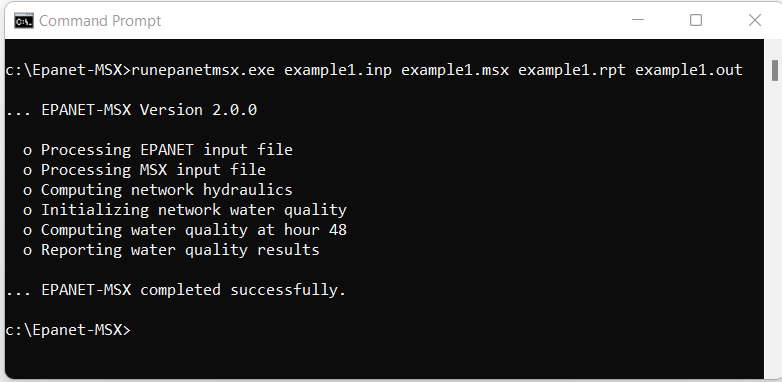
Fig. 3.2 Command line execution of EPANET-MSX.
After the program finishes, the example1.rpt file can be opened in any text editor (such as Windows Notepad) where its contents can be viewed. Excerpts from the results file are reproduced in Listing 3.3. The first page contains a summary of the standard EPANET options that were chosen for the run. Following this is a table of results for each node and each link. These tables contain the concentrations of each species at each reporting period. Note that the surface species are not listed for nodes since by definition this class of constituent is associated only with pipe surfaces. At the end of the report file, the mass balance summaries of the three differential variables (\(As^{+3}\), :\(As^{+5}\) and \(NH_2Cl\)) are provided. These mass balances reports are consistent with those provided by EPANET 2.2, and will include all relevant species. Starting and ending mass, mass inflow, outflow, and reacted are included.
  Page 1                                    Thu Feb  9 10:40:39 2023

  ******************************************************************
  *                           E P A N E T                          *
  *                   Hydraulic and Water Quality                  *
  *                   Analysis for Pipe Networks                   *
  *                         Version 2.2                            *
  ******************************************************************

  EPANET-MSX Example Network

      Input Data File ................... example1.inp
      Number of Junctions................ 4
      Number of Reservoirs............... 1
      Number of Tanks ................... 0
      Number of Pipes ................... 5
      Number of Pumps ................... 0
      Number of Valves .................. 0
      Headloss Formula .................. Hazen-Williams
      Nodal Demand Model ................ DDA
      Hydraulic Timestep ................ 1.00 hrs
      Hydraulic Accuracy ................ 0.001000
      Status Check Frequency ............ 2
      Maximum Trials Checked ............ 10
      Damping Limit Threshold ........... 0.000000
      Maximum Trials .................... 200
      Quality Analysis .................. None
      Specific Gravity .................. 1.00
      Relative Kinematic Viscosity ...... 1.00
      Relative Chemical Diffusivity ..... 1.00
      Demand Multiplier ................. 1.00
      Total Duration .................... 48.00 hrs
      Reporting Criteria:
         No Nodes
         No Links

  Analysis begun Thu Feb  9 10:40:39 2023

  Processing MSX input file example1.msx


Page 1                                               EPANET-MSX 2.0.0

  ******************************************************************
  *                      E P A N E T  -  M S X                     *
  *                   Multi-Species Water Quality                  *
  *                   Analysis for Pipe  Networks                  *
  *                           Version 2.0.0                        *
  ******************************************************************

  Arsenic Oxidation/Adsorption Example


  <<< Node C >>>

  Time            AS5       AStot       NH2CL
  hr:min         UG/L        UG/L        MG/L
  -------  ----------  ----------  ----------
     0:00        0.00        0.00        0.00
     2:00        0.00        0.00        0.00
     4:00        0.00        0.00        0.00
     6:00        0.00        0.00        0.00
     8:00        0.00        0.00        1.10
    10:00        9.17        9.17        1.10
    12:00        9.17        9.17        1.10
    14:00        9.17        9.17        1.10
    16:00        9.17        9.17        1.10
    18:00        9.17        9.17        1.10
    20:00        9.17        9.17        1.10
    22:00        9.17        9.17        1.10
    24:00        9.17        9.17        1.10
    26:00        9.17        9.17        1.10
    28:00        9.17        9.17        1.10
    30:00        9.17        9.17        1.10
    32:00        9.17        9.17        1.10
    34:00        9.17        9.17        1.11
    36:00        9.17        9.17        1.11
    38:00       10.03       10.03        1.11
    40:00       10.03       10.03        1.11
    42:00       10.03       10.03        1.11
    44:00       10.03       10.03        1.11
    46:00       10.03       10.03        1.11
    48:00       10.03       10.03        1.11

  <<< Node D >>>

  Time            AS5       AStot       NH2CL
  hr:min         UG/L        UG/L        MG/L
  -------  ----------  ----------  ----------
     0:00        0.00        0.00        0.00
     2:00        0.00        0.00        0.00
     4:00        0.00        0.00        0.00
     6:00        0.00        0.00        0.00
     8:00        0.00        0.00        0.00
    10:00        0.00        0.00        0.00
    12:00        0.00        0.00        0.00
    14:00        0.00        0.00        0.00
    16:00        0.00        0.00        0.00
    18:00        0.00        0.00        0.00
    20:00        0.00        0.00        0.00
    22:00        0.00        0.00        0.00
    24:00        0.00        0.00        0.24
    26:00        0.00        0.00        0.24
    28:00        9.17        9.17        0.24
    30:00        9.17        9.17        0.24
    32:00        9.17        9.17        0.24
    34:00        9.17        9.17        0.24
    36:00        9.17        9.17        0.24
    38:00        9.17        9.17        0.24
    40:00        9.17        9.17        0.24
    42:00        9.17        9.17        0.24
    44:00        9.17        9.17        0.24
    46:00        9.17        9.17        0.24
    48:00        9.17        9.17        0.24

  <<< Link 5 >>>

  Time            AS5       AStot        AS5s       NH2CL
  hr:min         UG/L        UG/L       UG/M2        MG/L
  -------  ----------  ----------  ----------  ----------
     0:00        0.00        0.00       -0.00        0.00
     2:00        0.00        0.00        0.00        0.00
     4:00        0.00        0.00        0.00        0.00
     6:00        0.00        0.00        0.00        0.00
     8:00        0.00        0.00        0.00        0.05
    10:00        0.85        0.85        4.51        0.17
    12:00        1.86        1.86        9.88        0.27
    14:00        2.87        2.87       15.27        0.35
    16:00        3.87        3.87       20.64        0.42
    18:00        4.88        4.88       26.02        0.47
    20:00        5.89        5.89       31.39        0.52
    22:00        6.89        6.89       36.75        0.55
    24:00        7.90        7.90       42.12        0.56
    26:00        8.91        8.91       47.50        0.56
    28:00        9.17        9.17       48.93        0.56
    30:00        9.17        9.17       48.93        0.56
    32:00        9.17        9.17       48.93        0.56
    34:00        9.17        9.17       48.93        0.56
    36:00        9.17        9.17       48.93        0.57
    38:00        9.19        9.19       48.93        0.57
    40:00        9.30        9.30       48.95        0.57
    42:00        9.41        9.41       48.96        0.57
    44:00        9.52        9.52       48.97        0.57
    46:00        9.64        9.64       48.98        0.57
    48:00        9.75        9.75       48.99        0.57


  Water Quality Mass Balance: AS3 (UG)
  ================================
  Initial Mass:       0.00000e+00
  Mass Inflow:        7.34409e+06
  Mass Outflow:       5.15609e-11
  Mass Reacted:      -7.32740e+06
  Final Mass:         1.66911e+04
  Mass Ratio:         1.00000
  ================================


  Water Quality Mass Balance: AS5 (UG)
  ================================
  Initial Mass:       0.00000e+00
  Mass Inflow:        0.00000e+00
  Mass Outflow:       5.79736e+06
  Mass Reacted:       7.13763e+06
  Final Mass:         1.34027e+06
  Mass Ratio:         1.00000
  ================================


  Water Quality Mass Balance: NH2CL (MG)
  ================================
  Initial Mass:       0.00000e+00
  Mass Inflow:        1.83602e+06
  Mass Outflow:       8.51117e+05
  Mass Reacted:      -8.00156e+05
  Final Mass:         1.84749e+05
  Mass Ratio:         1.00000
  ================================


  Analysis ended Thu Feb  9 10:40:39 2023
3.2. Example Toolkit Usage
Using the EPANET-MSX function library requires some programming effort to build custom applications and must be used in conjunction with the standard EPANET Programmer’s Toolkit. Applications can be written in any programming language that can call external functions residing in a Windows DLL (or a Linux shared object library), such as C, C++, Visual Basic, and Delphi Pascal. Section MSX TOOLKIT FUNCTIONS describes each function included in the MSX toolkit library. The functions in the EPANET toolkit library are documented online at http://wateranalytics.org/EPANET/.
As an example of how the library can be used to construct an application, Listing 3.4 displays the C code behind the command line implementation of the MSX system, runepanetmsx.exe, which was just discussed. The listing begins by checking for the correct number of command line arguments and then attempts to open and read the EPANET file supplied as the first argument. It uses the EPANET toolkit function ENopen for this purpose.
The code then begins a do-while loop that simplifies error detection through the remainder of the program. The MSXopen function is used to open and process the MSX file (the second command line argument), and the MSXsolveH function is used to run a hydraulic analysis of the network whose results are saved to a scratch file. This is followed by a call to MSXinit to initialize the water quality analysis. Note that the argument of 1 to this function tells the MSX system to save its computed water quality results to a scratch file so that they can be used for reporting purposes later on.
The program then begins another do-while loop that will step through each water quality time step. At each such step, the MSXstep function is called to update water quality throughout the network and save these results to the scratch output file. This function also updates the amount of time left in the simulation (stored in the variable named tleft). The loop continues until either no more time is left or an error condition is encountered.
If the simulation ends successfully, the MSXreport function is called to write the water quality results to the report file that was named on the command line. If a fourth file name was supplied on the command line, then the MSXsaveoutfile is called to save the results in a binary format to this file. Lastly, the MSX system is closed down by calling MSXclose and the same is done for the EPANET system by calling ENclose.
If the source code in Listing 3.4 was saved to a file named epanetmsx.c then it could be compiled into an executable named runepanetmsx.exe by first opening a Microsoft Visual Studio command prompt window (64-bit) and then using the following commands:
CL /c epanetmsx.c
LINK epanetmsx.obj epanet2.lib epanetmsx.lib /OUT:runepanetmsx.exe
Note that when developing MSX applications in C/C++, the header files epanet2.h, epanetmsx.h and epanet2_enums.h must be in the same folder as the application’s source codes (epanetmsx.c here), and the library modules epanet2.lib and epanetmsx.lib must be linked in with the application’s object modules. Versions of these files that are compatible with the Microsoft C/C++ compiler (Version 6 and higher) are supplied with the EPANET-MSX distribution. Also, copies of the distributed DLL files epanet2.dll and epanetmsx.dll must be placed in the same directory as the application’s executable file or reside in a directory listed the user’s PATH environment variable.
Users using other compilers or platforms would need to use the appropriate commands to produce the required object library files and executables.
//  EPANETMSX.C  -- Command line implementation of EPANET-MSX

#include <stdlib.h>
#include <stdio.h>
#include "epanet2.h"                   // EPANET toolkit header file
#include "epanetmsx.h"                 // EPANET-MSX toolkit header file

int main(int argc, char* argv[])
/*
**  Purpose:
**    runs a multi-species EPANET analysis
**
**  Input:
**    argc = number of command line arguments
**    argv = array of command line arguments.
**
**  Returns:
**    an error code (or 0 for no error).
**
**  Notes:
**    The command line arguments are:
**     - the name of a regular EPANET input data file
**     - the name of a EPANET-MSX input file
**     - the name of a report file that will contain status
**       messages and output results
**     - optionally, the name of an output file that will
**       contain water quality results in binary format.
*/
{
    int    err, done = 1;
    double   t, tleft;
    long   oldHour, newHour;

    // --- Check command line arguments

    if (argc < 4) {
        printf("\n Too few command line arguments.\n");
        return 0;
    }
    // --- Open the EPANET file

    printf("\n... EPANET-MSX Version 2.0\n");
    printf("\n  o Processing EPANET input file");
    err = ENopen(argv[1], argv[3], "");
    if (err) {
        printf("\n\n... Cannot read EPANET file; error code = %d\n", err);
        ENclose();
        return 0;
    }
    // ---  Begin an error detection loop

    do {

        // --- Open the MSX input file

        printf("\n  o Processing MSX input file");
        err = MSXopen(argv[2]);
        if (err) {
            printf("\n\n... Cannot read MSX file; error code = %d\n", err);
            break;
        }

        // --- Solve hydraulics

        printf("\n  o Computing network hydraulics");
        err = MSXsolveH();
        if (err) {
            printf(
                "\n\n... Cannot obtain network hydraulics; error code = %d\n", err);
            break;
        }

        // --- Initialize the multi-species analysis

        printf("\n  o Initializing network water quality");
        err = MSXinit(1);
        if (err) {
            printf(
                "\n\n... Cannot initialize EPANET-MSX; error code = %d\n", err);
            break;
        }
        t = 0;
        oldHour = -1;
        newHour = 0;
        printf("\n");

        // --- Repeat for each time step

        do {

            // --- Report current progress
            if (oldHour != newHour) {
                printf("\r  o Computing water quality at hour %-4d", newHour);
                oldHour = newHour;
            }

            // --- Compute water quality
            err = MSXstep(&t, &tleft);
            newHour = (long) (t / 3600.0);

        } while (!err && tleft > 0);
        // --- Report any runtime error

        if (err) {
            printf("\n\n... EPANET-MSX runtime error; error code = %d\n", err);
            break;
        }
        else
            printf("\r  o Computing water quality at hour %-4d", (long) (t / 3600.0));

        // --- Report results

        printf("\n  o Reporting water quality results");
        err = MSXreport();
        if (err) {
            printf(
                "\n\n... MSX report writer error; error code = %d\n", err);
            break;
        }

        // --- Save results to binary file if a file name was provided

        if (argc >= 5) {
            err = MSXsaveoutfile(argv[4]);
            if (err > 0) {
                printf(
                    "\n\n... Cannot save MSX results file; error code = %d\n", err);
                break;
            }
        }

        // --- End of error detection loop

    } while (!done);

    // --- Close both the multi-species & EPANET systems

    MSXclose();
    ENclose();
    if (!err) printf("\n\n... EPANET-MSX completed successfully.");
    printf("\n");
    return err;
}
3.3. Using Compiled Reaction Models
EPANET-MSX has the option to compile the chemical reaction equations that a user specifies within their MSX input file using a C compiler that already resides on the user’s system. This can speed up execution times by a factor of 2 to 5, depending on the nature of the reaction system and the choice of integration method. This option is available on Windows operating systems that have either the Microsoft Visual Studio C++ compiler or the MinGW port of the Gnu C++ compiler installed, or on Linux systems with the Gnu C++ compiler. To utilize this option, one adds the following command to the [OPTIONS] (Section 4.2) section of the MSX input file:
COMPILER choice
where choice is VC for the Visual Studio C++ compiler, GC for the MinGW or Gnu C++ compilers, or NONE for no compiler (the default compiler option). To determine if your Windows system has the Visual Studio C++ build tools installed you can check to see if a Visual Studio folder appears on your Start Menu. To check for the MinGW compiler, open a Command Prompt window and enter gcc.
The Gnu compiler comes standard with most Linux installations.